Analyze
This area offers a set of techniques for data analysis.
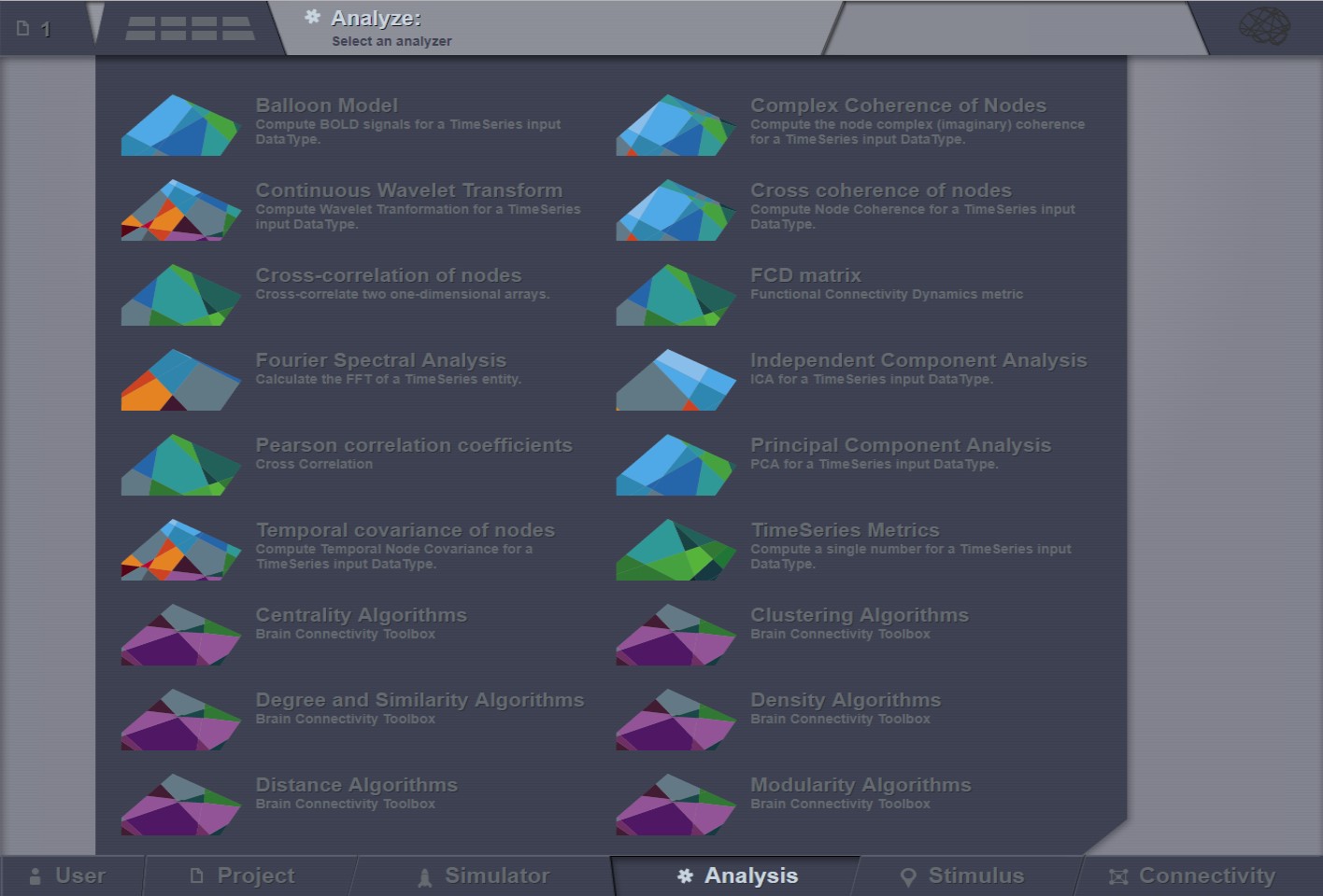
Current available analyzers
The Analyzers in TheVirtualBrain are not always the best implementations of the algorithms in terms of performance, neither are we offering a complete analysis spectrum, because analysis is not considered the focus feature of TheVirtualBrain and we do not intend to offer a replacement for tools already existent and successful in this area. We are merely offering some handy tools for people who want to directly process simulation results inside TheVirtualBrain, although the advised long term strategy is to export simulated data from TheVirtualBrain and analyze it intensively with specialized tools for your area of interest. We advise you not to run our analysis algorithms with long timeseries, as some might take a lot of time to finish.
The Analysis area has several interfaces that support the following operations for time-series analysis (and not only):
Cross-correlation of nodes
Fourier Spectral Analysis
Global TimeSeries Metrics
Cross coherence of nodes
Temporal covariance of nodes
Principal Component Analysis
Independent Component Analysis
Continuous Wavelet Transform
Cross-correlation of nodes
Compute pairwise temporal cross-correlation of all nodes in a 4D TimeSeries object. Cross-correlation, or normalized cross-covariance, is a measure that quantifies the degree of linear dependence between two time-series.
To calculate the correlation coefficient of all nodes of a given multi-node time-series, simply select the TimeSeries object from the drop-down list in the Cross-correlation of nodes interface and hit Launch.
The algorithm returns a CrossCorrelation object that contains cross correlation coefficients for all possible combinations of nodes. Results are visualized with the Correlation viewer.
Fourier Spectral Analysis
Compute a fast Fourier transform (FFT) of a TimeSeries object. FFT is an algorithm to compute the discrete Fourier transform (DFT) and its inverse for a 1 given sequence of values. DFT transforms a function into its frequency-domain representation, that is, a sum of weighted sinusoids while preserving all of the information about the original signal. After decomposing the signal, spectrum analysis quantifies the relative amounts of amplitudes, powers, intensities or phases of a component versus its frequency.
In order to perform a Fourier analysis of your time-series data follow these steps:
Go to the Fourier Spectral Analysis interface and select a Windowing function, you can choose among ‘hamming’, ‘bartlett’, ‘blackman’ and ‘hanning’.
Select the time-series.
Select a segment length.
Hit Launch.
TimeSeries Metrics
Calculate one scalar metric to characterize the time-series dataset.
Cross coherence of nodes
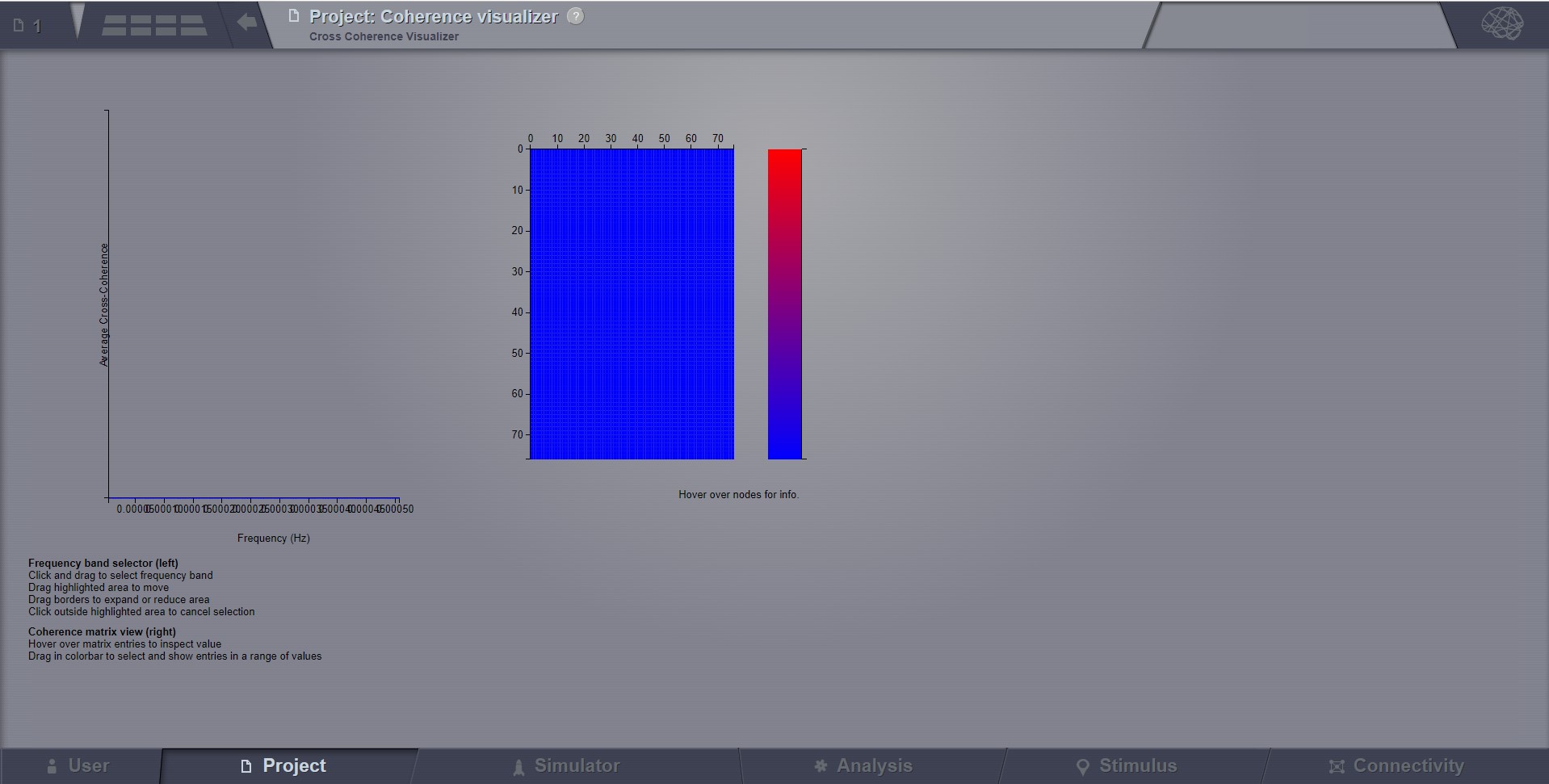
Calculate pairwise temporal coherence of all nodes in a 4D TimeSeries object. Coherence analysis, or cross-spectral analysis, can be used to estimate how two time series are related in the spectral domain. Cross-coherence indicates the degree to which amplitude and phase between two signals relate to each other as a function of frequency.
To calculate the cross-coherence of all nodes of a given multi-node time-series, simply select the TimeSeries object from the drop-down list in the Cross coherence of nodes interface, select an appropriate measure for data-point per block, and hit Launch.
The resulting coherence spectrum can be viewed with the Cross coherence visualizer.
Complex coherence of nodes
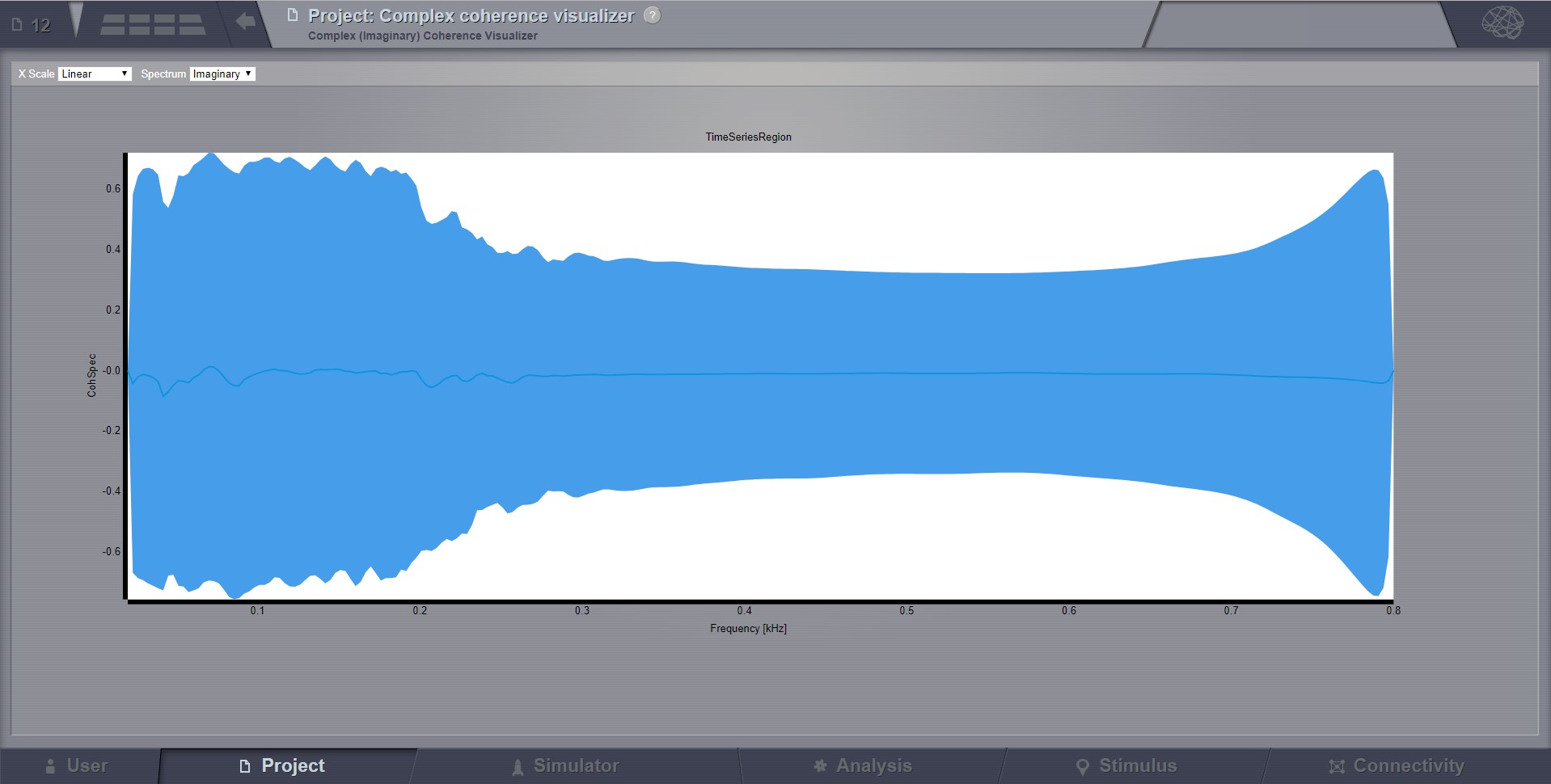
To calculate the complex-cross-coherence of all nodes of a given multi-node time-series, simply select the TimeSeries object from the drop-down list in the Complex coherence of nodes interface and hit Launch.
The resulting coherence spectrum can be viewed with the Complex coherence visualizer.
Temporal covariance of nodes
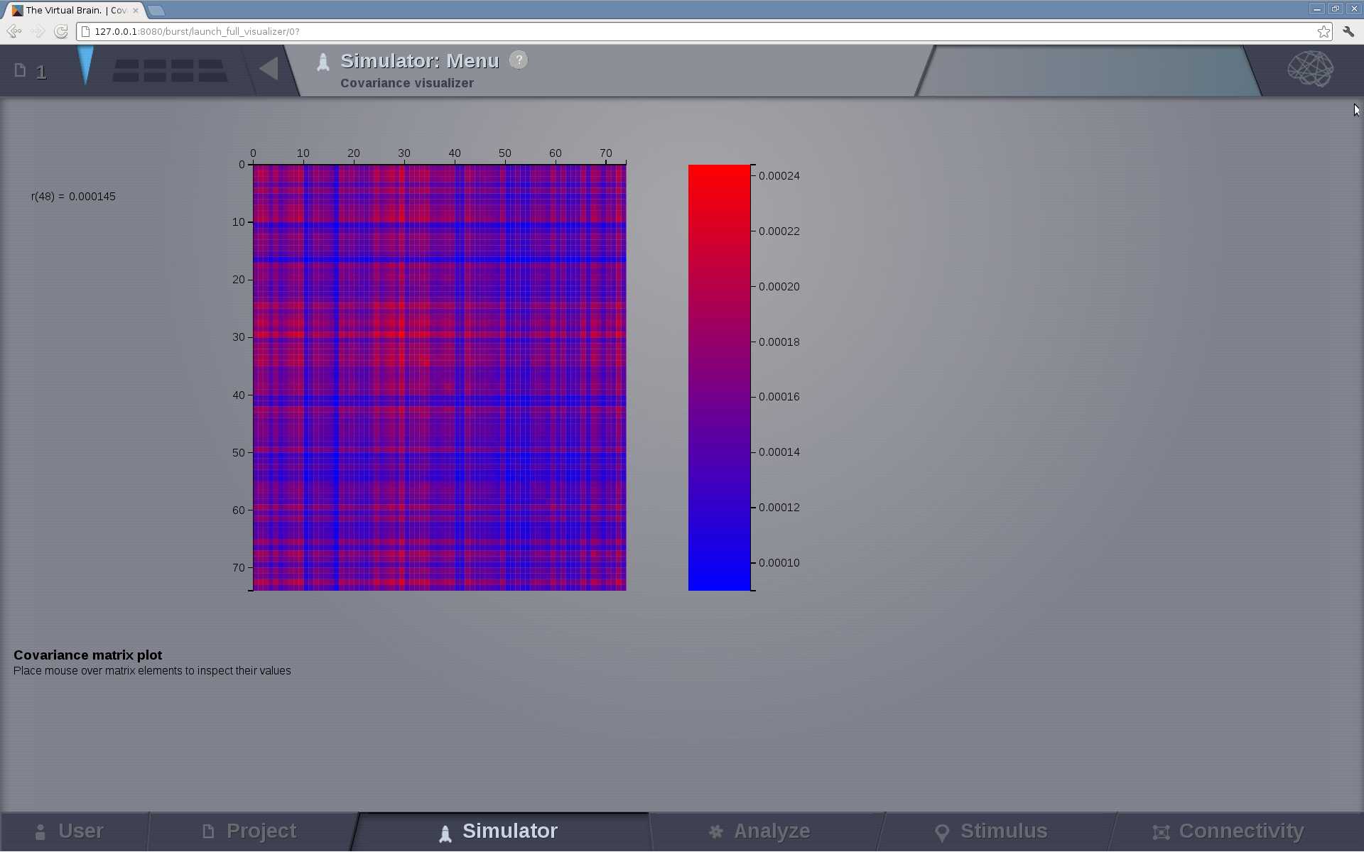
Compute pairwise temporal covariance of all nodes in a 4D TimeSeries object. Covariance resembles the un-normalized correlation coefficient and measures how much two time-series change together.
To calculate the temporal covariance of all nodes of a given multi-node time-series, select the TimeSeries object from the drop-down list in the Independent Component Analysis interface and hit Launch.
The algorithm returns a Covariance object that is a 4D-Matrix with the Dimensions {nodes, nodes, 1, 1}. The resulting covariance matrix can be viewed with the Covariance visualizer.
Principal Component Analysis (PCA)
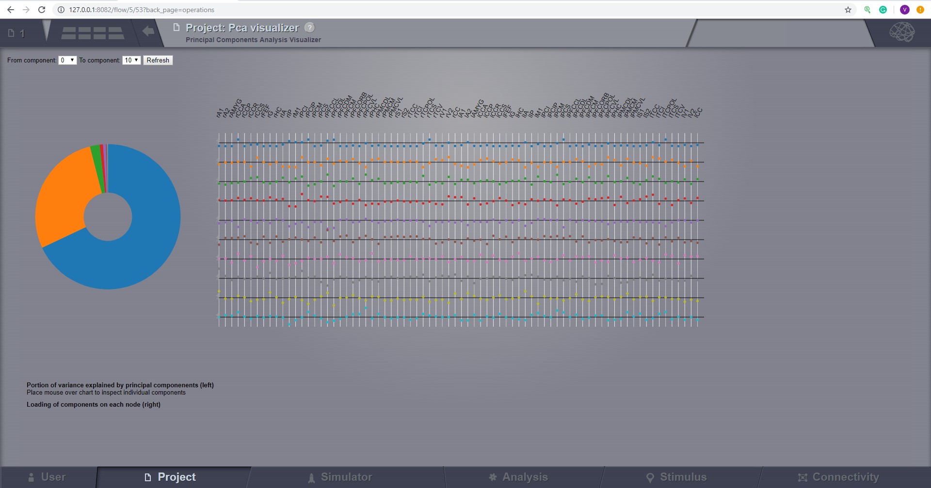
Compute a PCA of a 4D TimeSeries object. PCA is a computational method for multivariate data analysis that uses an orthogonal transformation to convert a set of (possibly correlated) variables into a set of linearly uncorrelated variables called principal components.
To calculate a PCA of all nodes of a given multi-node time-series, select the 4D-TimeSeries object from the drop-down list in the Principal Components Analysis interface and hit Launch.
The algorithm returns an PrincipalComponents object that is a xD-Matrix with the Dimensions {x,y,z}. The resulting time-series can be viewed with the Pca viewer.
Independent Component Analysis (ICA)
Compute a time-domain ICA decomposition of a 4D TimeSeries object. ICA is a statistical and computational method for separating a multivariate signal into additive subcomponents by maximizing the mutual statistical independence of source signals.
To calculate a temporal ICA of all nodes of a given multi-node time-series, select the 4D-TimeSeries object from the drop-down list in the Independent Component Analysis interface and hit Launch.
The algorithm returns an IndependentComponents object that is a xD-Matrix with the Dimensions {x,y,z}. The resulting time-series can be viewed with the corresponding ICA viewer.
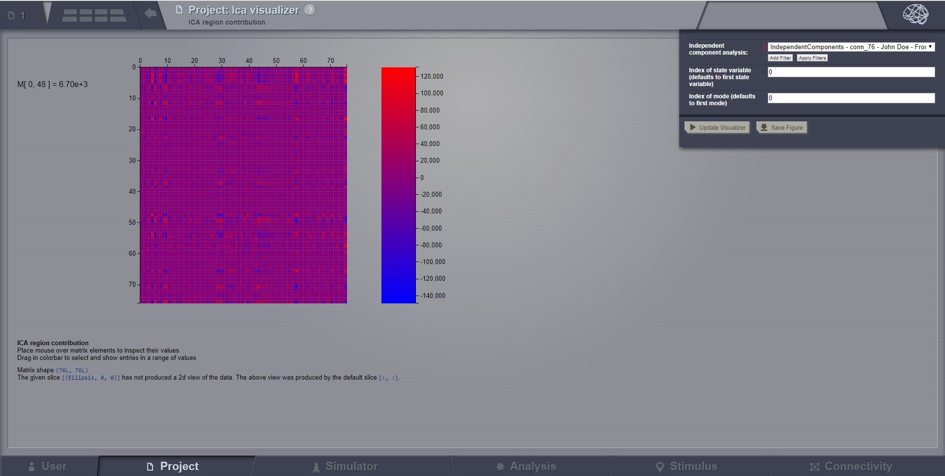
Preview for Independent Components Analysis Visualizer
Continuous Wavelet Transform (CWT)
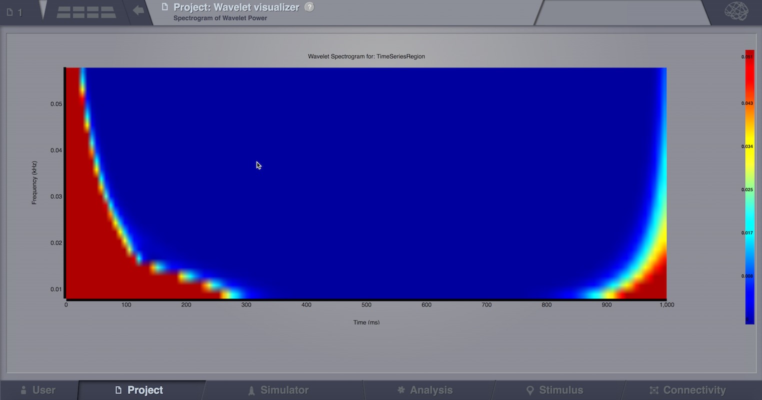
Compute a CWT of a 4D TimeSeries object. CWT decomposes a signal into wavelets of different frequencies yielding a time-frequency representation of the signal.
To calculate a CWT of all nodes of a given multi-node time-series, select the 4D-TimeSeries object from the drop-down list in the Continuous Wavelet Transform interface, specify transformation parameters like:
mother wavelet function
frequency resolution and range
type of the normalization for the resulting wavelet spectrum
Q-ratio
Sampling period of the spectrum
and hit Launch.
The algorithm returns an WaveletCoefficients object that is a xD-Matrix with the Dimensions {x,y,z}. The resulting spectrogram of wavelet power can be viewed with the Wavelet viewer.
Brain Connectivity Toolbox Analyzers
All the algorithms offered by Brain Connectivity Toolbox (BCT) can be used directly from TheVirtualBrain interface and the results can later be displayed in one of our visualizers.
Additional BCT techniques are:
Degree and Similarity Algorithms
Centrality Algorithms
Distance Algorithms
Modularity Algorithms
Clustering Algorithms
Density Algorithms
For more details, please refer to BCT web site
Functional Connectivity Dynamics metric
Analyse functional connectivity dynamics.
The analyser generates:
The FCD
The FCD segmented, that is the FCD matrix with the entries corresponding to the time points not belonging to the epochs of stability equal to 1.1. When the epochs of stability are not find, the FCD segmented is not an output
The 3 eigenvectors corresponding to the FC of the epochs (if present) or to the global FC. These are ConnectivityMeasures which are viewable with the volume visualizer.
The analyser takes as input a time series region, time window length (in ms), spanning between 2 consecutive time windows (in ms).
The code does the following steps:
- Calculates the FCD:
The entire time series is divided in time window of the fixed length (decided by the user) and with an overlap decided by the user ( spanning=[time window length] - [overlapping between consecutive time window]). The data points within each window, centred at time ti, are used to calculate FC(ti). The element ij of the FCD is calculated as the Pearson correlation between the upper triangular part of FC(ti) arranged as a vector and the upper triangular part of FC(tj) arranged as a vector.
- The FCD is segmented in epochs of stability using the spectral embedding algorithm.
We call epoch of stability a length of time during which an FC configuration stays stable. It is possible to visualize these epochs of stable FC as blocks of elevated inter-FC(t) correlation around the diagonal of the FCD. We neglect always the first epoch of stability found by the algorithm since should be an artifact caused by the initial condition of the simulated time series.
- FCs are calculated over the epochs of stability (excluding the first epoch).
When the algorithm does not find the epochs the global FC is calculated, i.e. the FC calculated over the entire timeseries.
- The first three eigenvectors of the FCs calculated at step 3 are extracted.
We call the “first” eigenvector the one associated to the largest eigenvalue, the second eigenvector the one associated to the second largest eigenvalue and so on. Eigenvalues are normalized between 0 and 1.