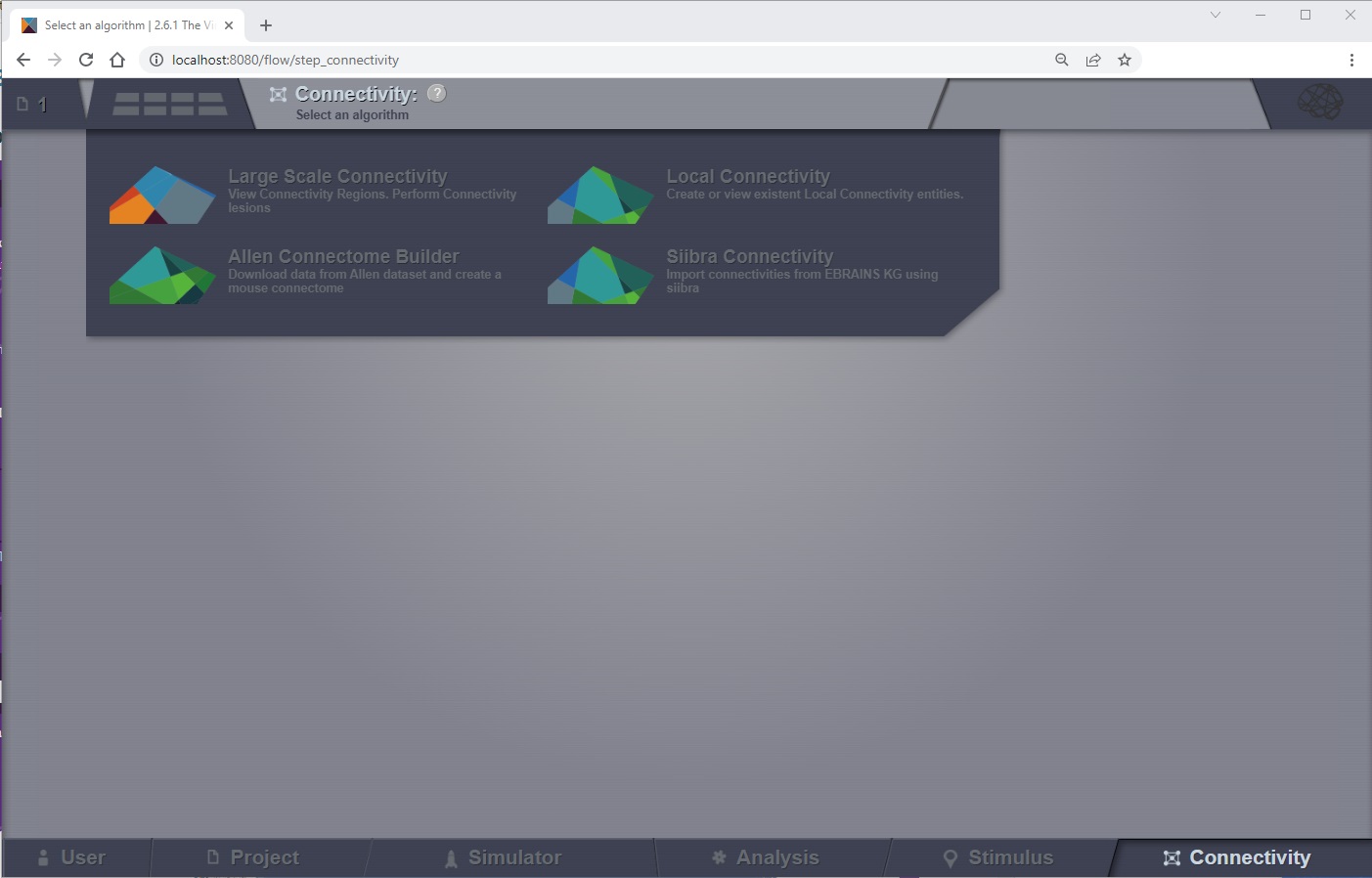
In this area you can edit two types of TVB connectivity objects:
long-range connectivity and,
local connectivity.
You can also download connectomes from the Allen Mouse Brain Connectivity Atlas or create structural and
functional connectivities with data from the EBRAINS Knowledge Graph using the siibra library.
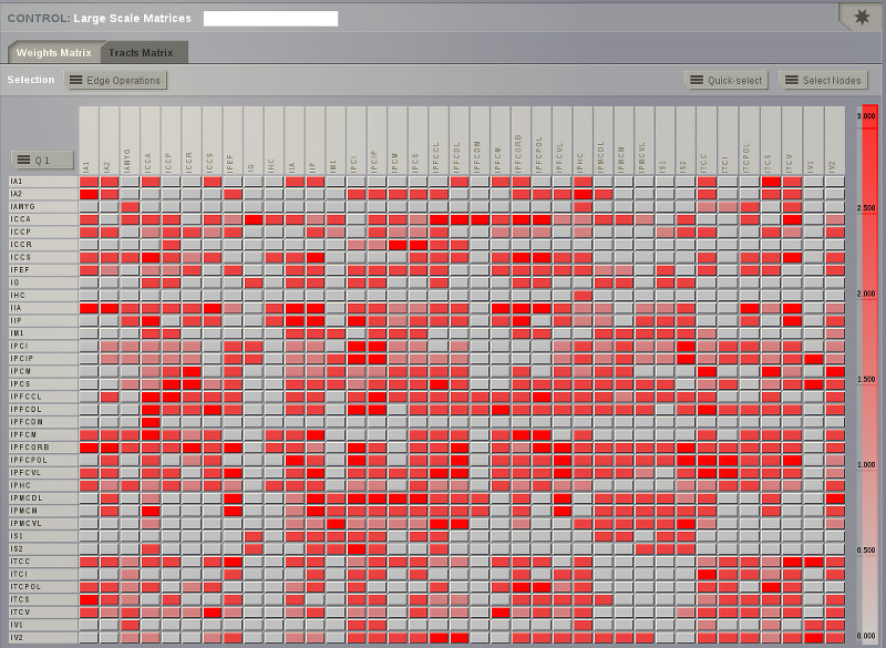
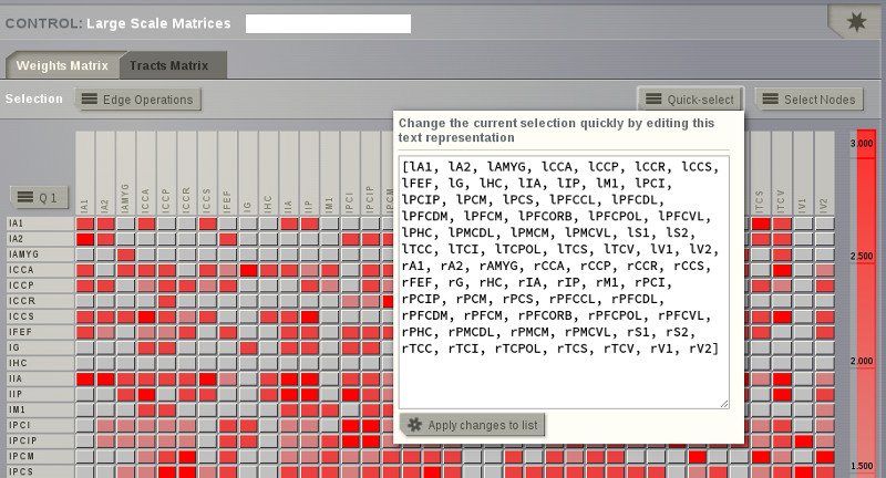
easily edit the connectivity weights or tract lengths
select a subset of the available nodes
perform basic algebraic operations on that group; and
save the new version as a new connectivity matrix.
The Connectivity datatype will be available in the Simulator area.
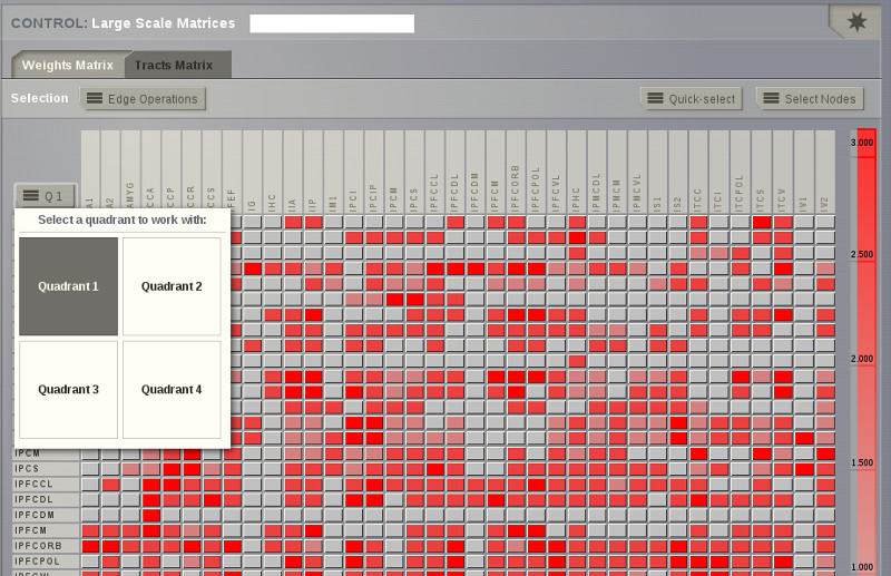
Hint
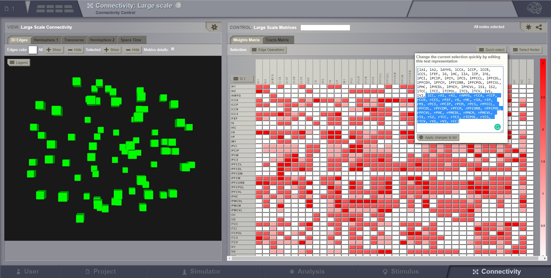
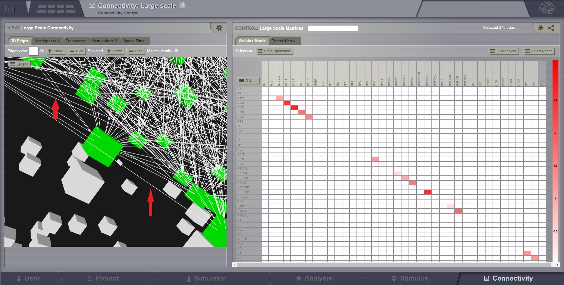
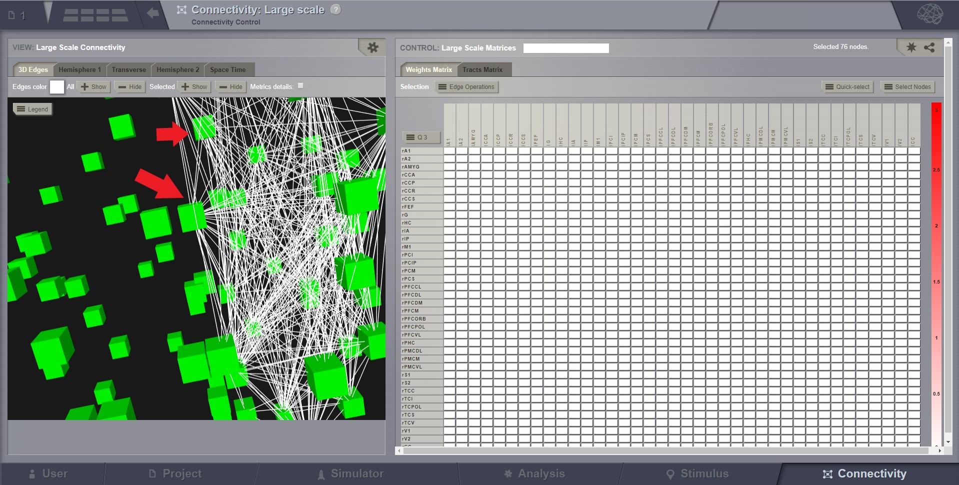
In the Connectivity Editor only one quadrant is displayed at a time.
You can select which quadrant is shown by accessing the quadrant selector
button in the upper left corner of the matrix display.
Assuming that the connectivity matrix is sorted such that the first half
corresponds one single hemisphere:
quadrants 1 and 4 will represent the intra-hemispheric connections,
and quadrants 2 and 3 will be the inter-hemispheric connections.
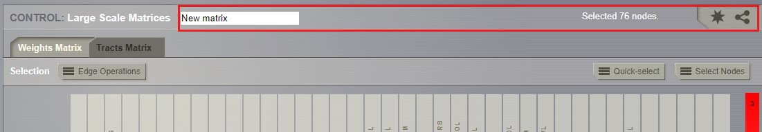
TVB enables you to save a new Connectivity object by clicking on .
This entity can be used later on in TheVirtualBrain Simulator.
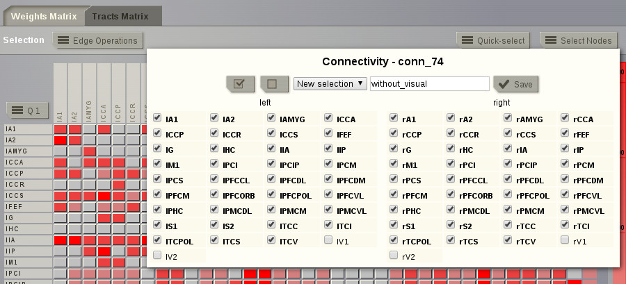
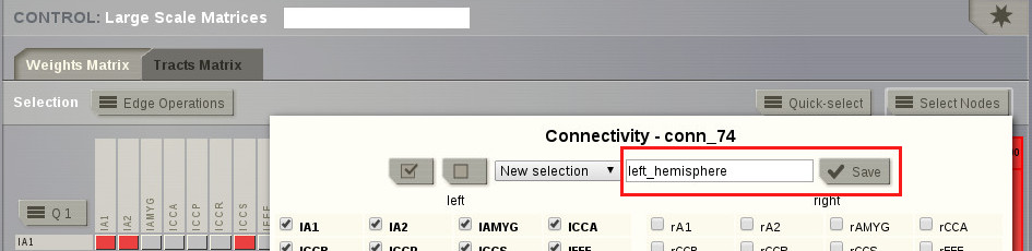
You can save a particular selection. Click the Select Nodes button and the selection component will be shown.
Enter a name for the selection and click save.
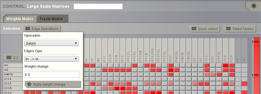
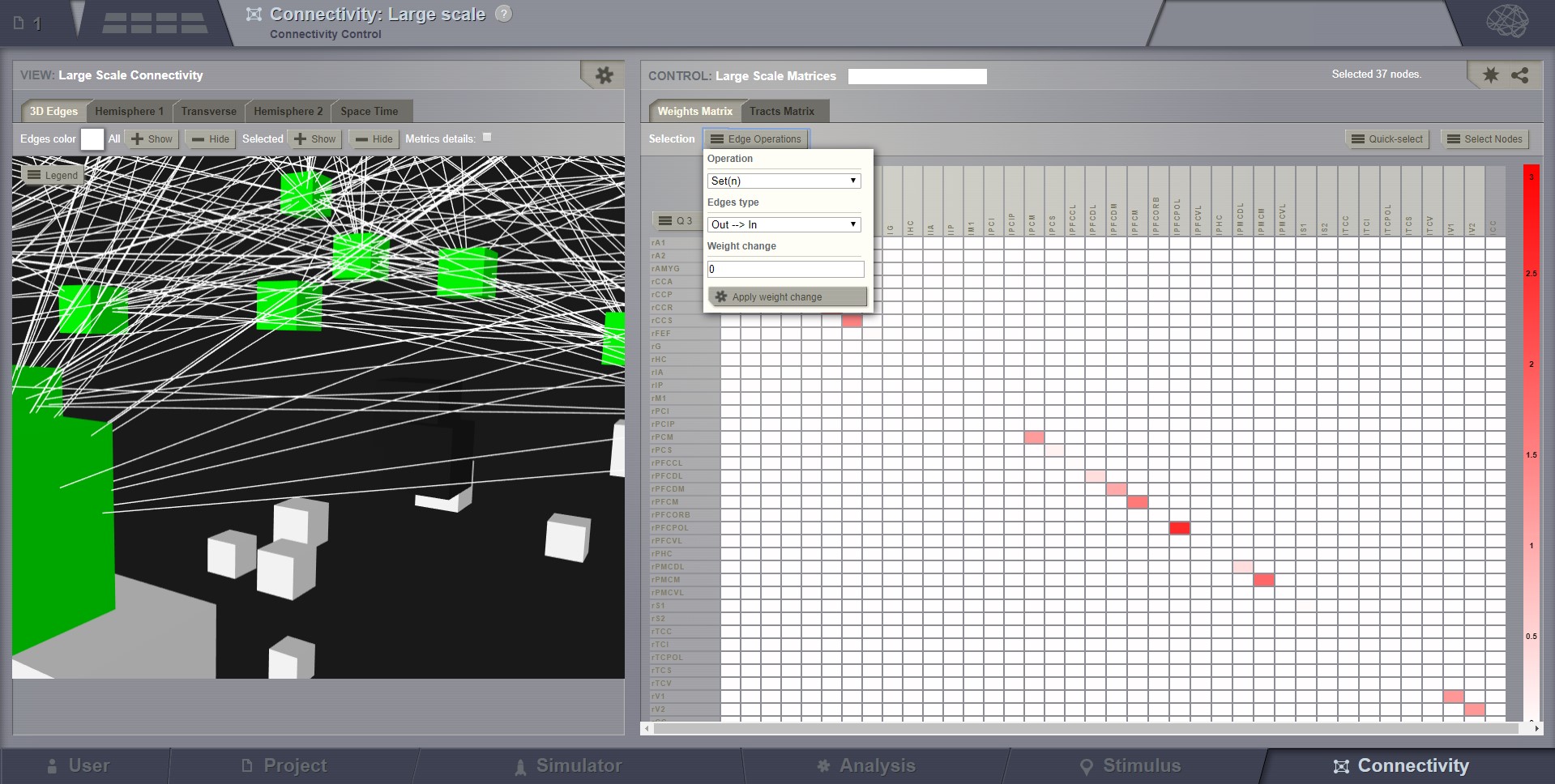
The Weights button opens a menu to perform basic algebraic operations on
a group of edges. You can select multiple nodes from the current connectivity
(by default all nodes are selected); thus you will end up with two sets of
nodes: the set of selected nodes and the set of un-selected nodes. These two
sets of nodes, determine four categories of edges:
In –> In: are only the edges connecting the nodes of the selected set.
In –> Out: are the edges that connect nodes in the selected set (rows) to nodes in the unselected set (columns).
Out –> In: are the edges connecting nodes in the unselected set (rows) to nodes in the selected set (columns).
Out –> Out: are edges connecting pair of nodes in the ‘unselected set’.
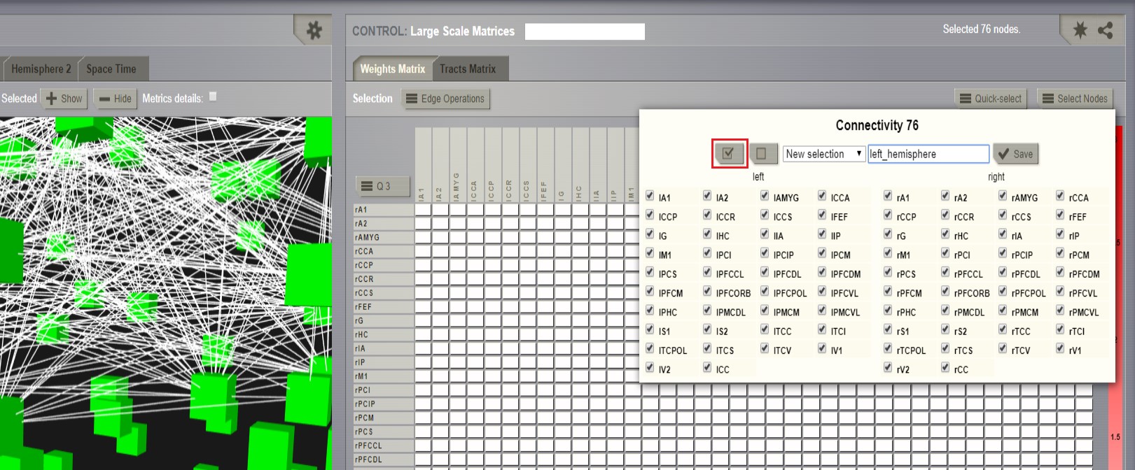
The inter-hemispheric connections are gone. Do not forget to select all the nodes again before saving your new matrix.
To do so click the select all button in the selection dropdown.
TVB is designed to handle connectivity matrices whose values are:
positive real values, meaning that there is a connection, or
zero values, meaning the absence of a connection
Warning
TVB does not handle unknowns such as NaNs or Infs.
If your connectivity matrix contains negative values, such as -1 values
you should either set these values to zero or an estimated value based
on your research assumptions.
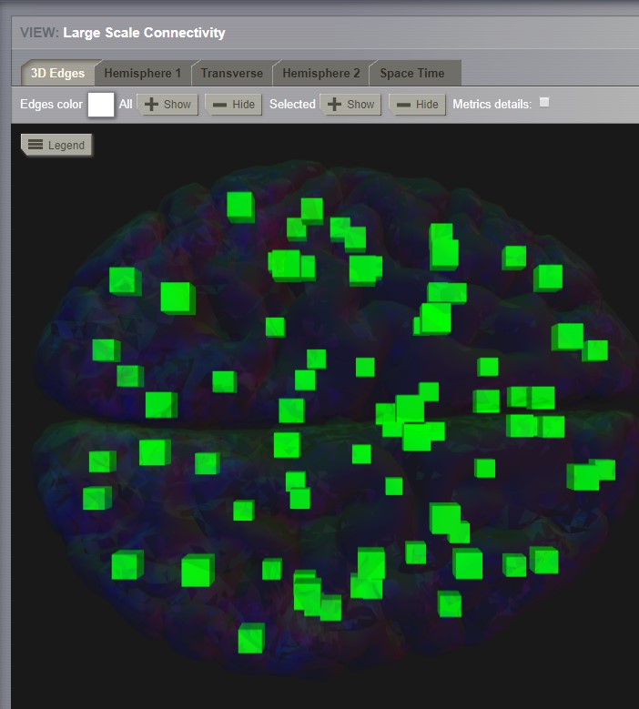
The 3D semi-transparent surface around the connectivity nodes, whether it is
the cortical surface or the outer-skin, is used just for giving space guidance.
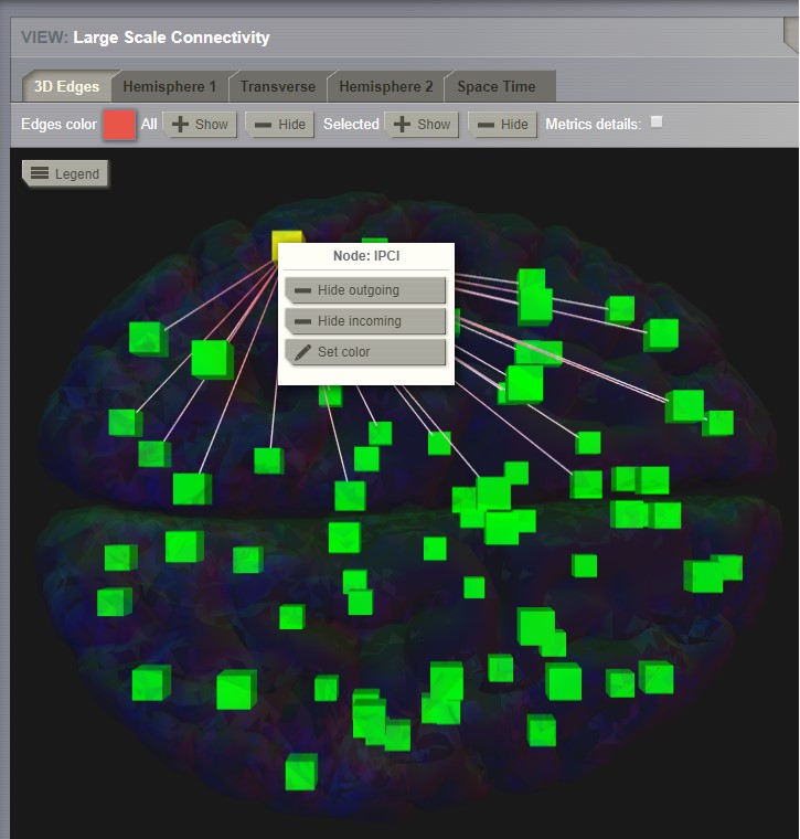
You can select an individual node and right-click on it to activate the incoming
or outgoing edges.
For each node you can choose a different color to apply to its
edges.
Preview for Connectivity Viewer 3D Edges - Coloring incoming / outgoing edges
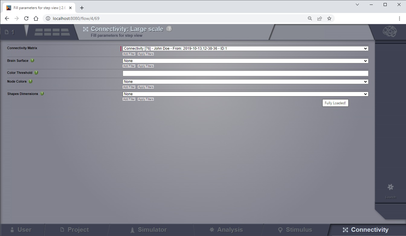
The 3D and 2D Views can be used to visualize two ConnectivityMeasure datatypes.
These measures can be the output of a BCT Analyzer.
If given, they will determine the size and colors of the nodes in the views.
You can choose these connectivity measures before launching the Large Scale Connectivity visualizer, or from the brain menu (see tip below).
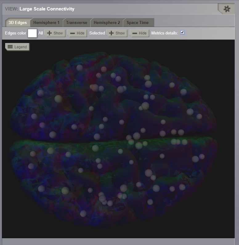
To display the measures in the 3D view check the Metrics details checkbox.
Nodes will be displayed as colored spheres. The size of the sphere is proportional to the measure labeled Shapes Dimensions.
The color comes from the current color scheme and is determined by the measure labeled Node Colors.
3D view of a connectivity measure. Node size is defined
by the Indegree. Node color is defined by node strength.
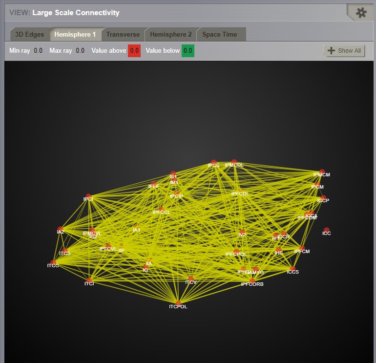
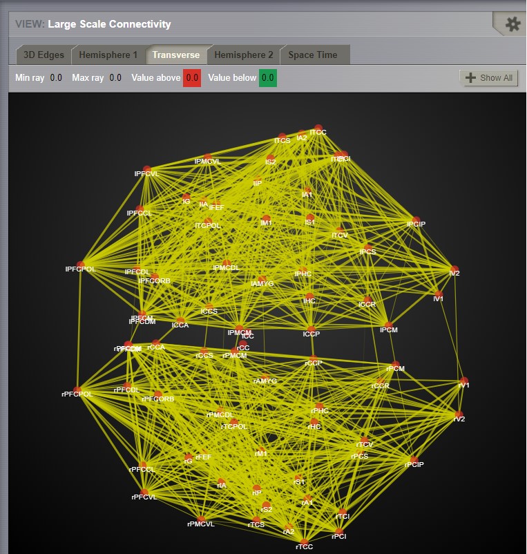
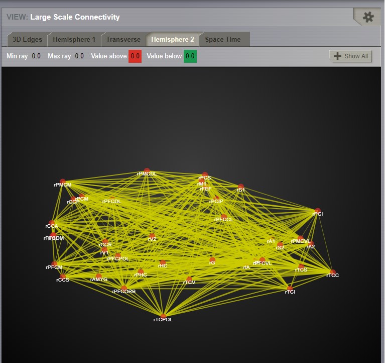
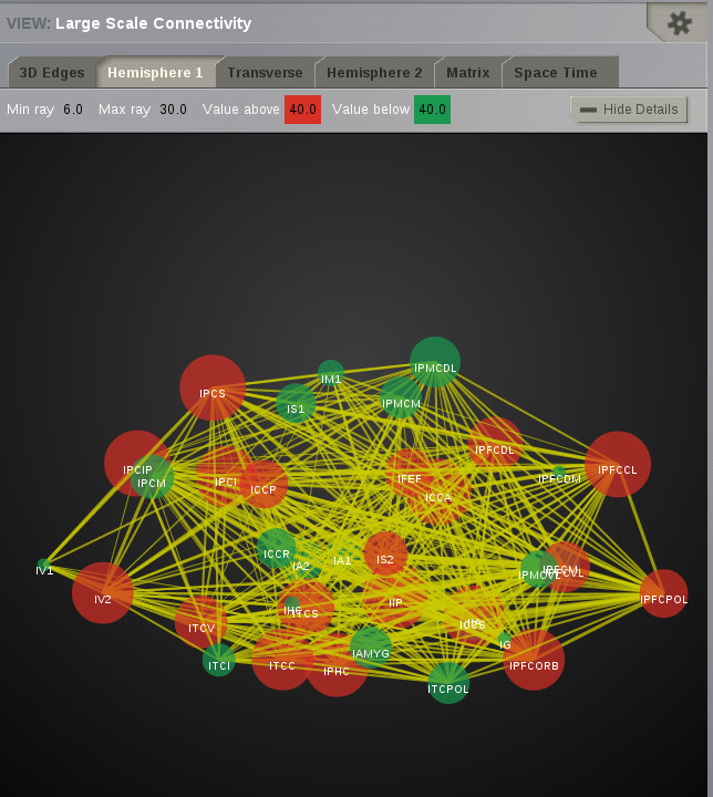
To display the measures in the 2D views click the Show all button.
Nodes are draws as circles, their size proportional to the measure labeled Shapes Dimensions.
Their color is determined by a threshold and the measure labeled Node Colors.
Nodes with values above the threshold will be red and those whose value are below the threshold will be green.
Preview of 2D Connectivity Viewer (left lateral view). Node size is defined
by the Indegree. Node color is defined by node strength, threshold is 40.
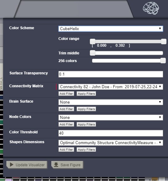
Tip
If you wish to change:
the color threshold,
the metrics used to define the node features,
the colormap used in the Connectivity Matrix Editor, or
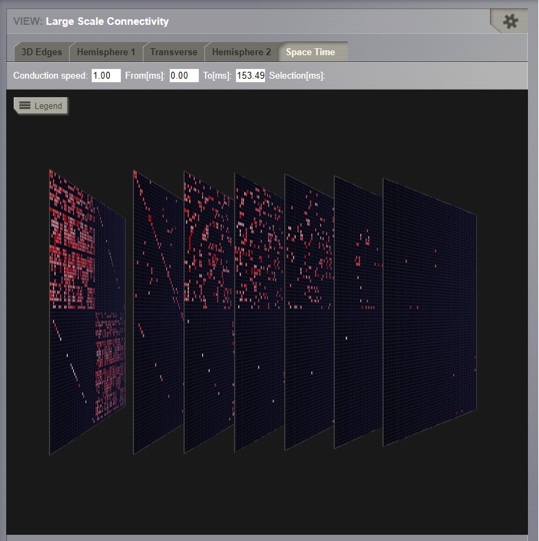
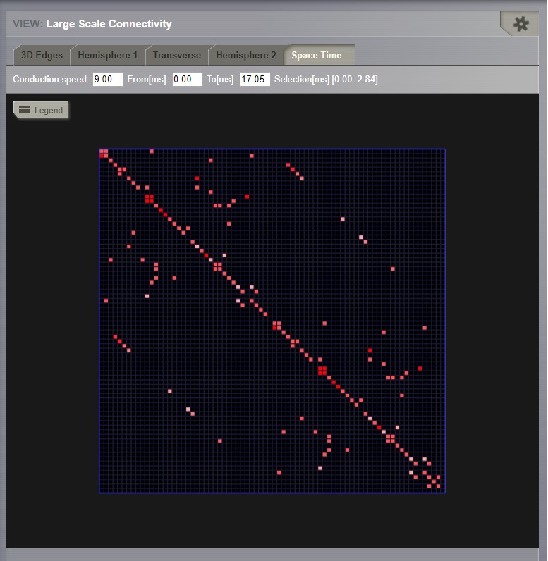
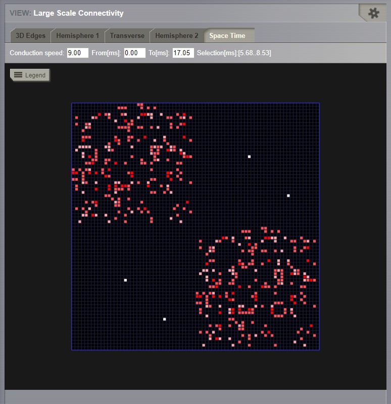
This is a three-dimensional representation of the delayed-connectivity
structure (space-time) when combined with spatial separation and a finite
conduction speed. The connectome consists of the weights matrix giving the
strength and topology of the network and the tract lengths matrix gives the
distance between pair of regions. When setting a specific conduction speed,
the distances will be translated into time delays. The space-time visualizer
disaggregate the weights matrix and each slice corresponds to connections
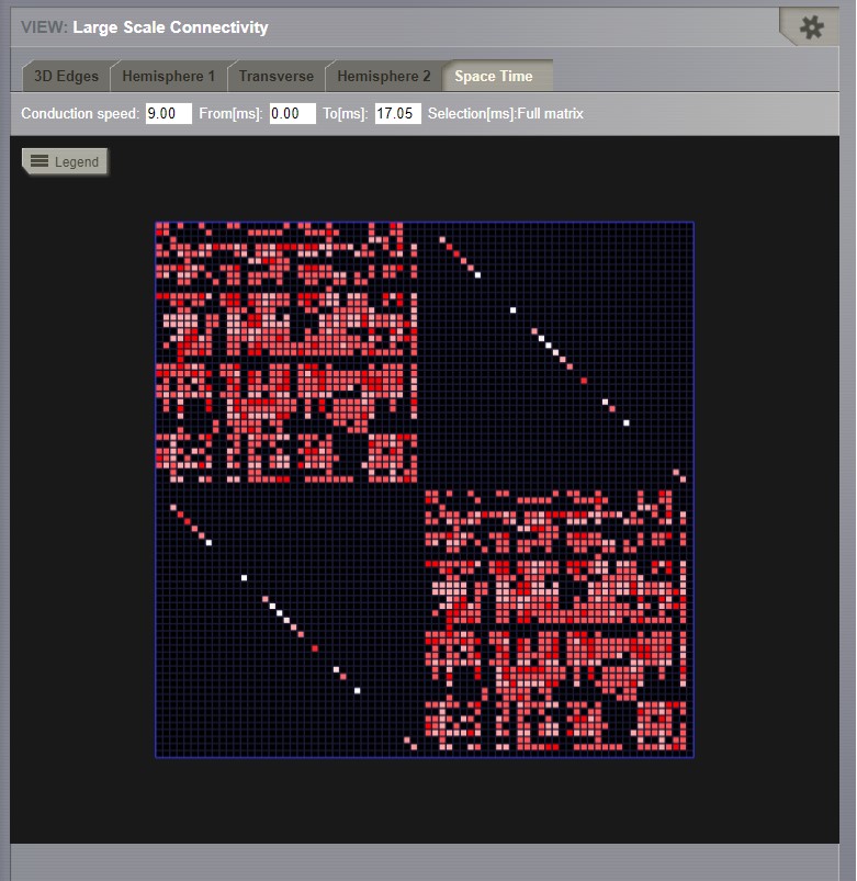
that fall into a particular distance (or delay) range. The first slice is the
complete weights matrix. Click on any of the subsequent slices to see the
corresponding 2D matrix plot.
From this page you can initiate an operation which will download data from The Allen Mouse Brain Connectivity Atlas.
See http://connectivity.brain-map.org
This operation needs an internet connection and it will take many minutes to complete.
It will produce a Structural Connectivity in TVB format and a compatible brain Volume object.
Check the Project –> Operations page to see when the import from Allen is done.
You can also find your resulted Connectivity in Project –> Data Structure area.
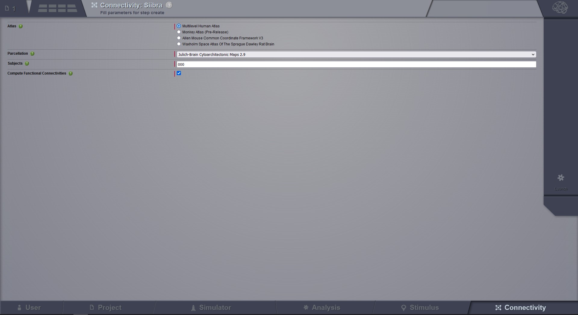
In this page you can use the siibra library
to create structural and functional connectivities using data from
to the EBRAINS Knowledge Graph. This knowledge graph
brings together information from different data sources regarding
brain atlases, parcellations and their associated features for multiple species. To be able to access
this information, you will need a special token provided by the EBRAINS team.
For more information, please refer to this page.
Currently, the structural connectivities are stored as TVB Connectivities and the
functional connectivities are stored as TVB Connectivity Measures.
In order to use the functionalities provided in this page, an internet connection is
required. Four parameters need to be configured in order to obtain structural and
functional connectivities, all of which come with default values for first time users.
For the atlas and parcellation parameters, you can see all the available options
through siibra. Selecting an atlas and a parcellation which are incompatible with
each other will result in an error after launching the operation.
The subjects field lets you specify the ids of the subjects for which you wish
to create the connectivities. The ids can be specified in 3 ways:
Individual ids, separated by ‘;’. For example: “000;001” will create
connectivities for subjects 000 and 001.
Range of ids, using ‘-’. For example: “000-002” will create
connectivities for subjects 000, 001 and 002.
Combination of the 2 aforementioned methods. For example: “000-002;100”
will create connectivities for subjects 000, 001, 002 and 100.
The last parameter, Compute Functional Connectivities, which comes in form
of a checkbox, lets you decide whether or not you wish to also extract the
functional connectivities from the Knowledge Graph. In case the box is checked,
5 functional connectivities will be created for each selected subject.
After pressing the Launch button, check the Project –> Operations page to see the
status of this operation. If it finished without an error, you will see there
the results: Connectivities and, optionally, Connectivity Measures. You can also
access the results from the Project –> Data Structure area.