Building Your Own Brain Network Model
TVB allows for a systematic exploration and manipulation of every underlying component of a large-scale brain network model, such as the neural mass model governing the local dynamics or the structural connectivity constraining the space-time structure of the network couplings.
Objectives
This tutorial presents the basic anatomy of a brain network model at the region level using The Virtual Brain’s (TVB’s) graphical interface. You are not expected to launch all the simulations.
We will be using the Default Project that should be imported when you start TVB. We’ll only go through the necessary steps required to reproduce some simulations. You can always start over, click along and/or try to change parameters.
Building A Discrete Brain Network Model
A basic simulation at the region level uses a coarse representation of the brain and consists of five main components, each of these components is a configurable object in TVB:
Model or Local population model, which is, at its core, a set of differential equations describing the local neuronal dynamics;
Connectivity, represents the large scale structural connectivity of the brain, i.e. white-matter tracts;
Long range Coupling, is a function that is used to join the local dynamics at distinct locations over the connections described in Connectivity;
Integrator, is the integration scheme that will be applied to the coupled set of differential equations;
Monitors, one or more Monitors can be attached to a simulation, their role is to record the output data.
In this example, we will change the default parameters to have a quick idea of some properties of the simulated data.
Go to the simulator page.
You can move through the fragments by clicking on the Next and Previous buttons.
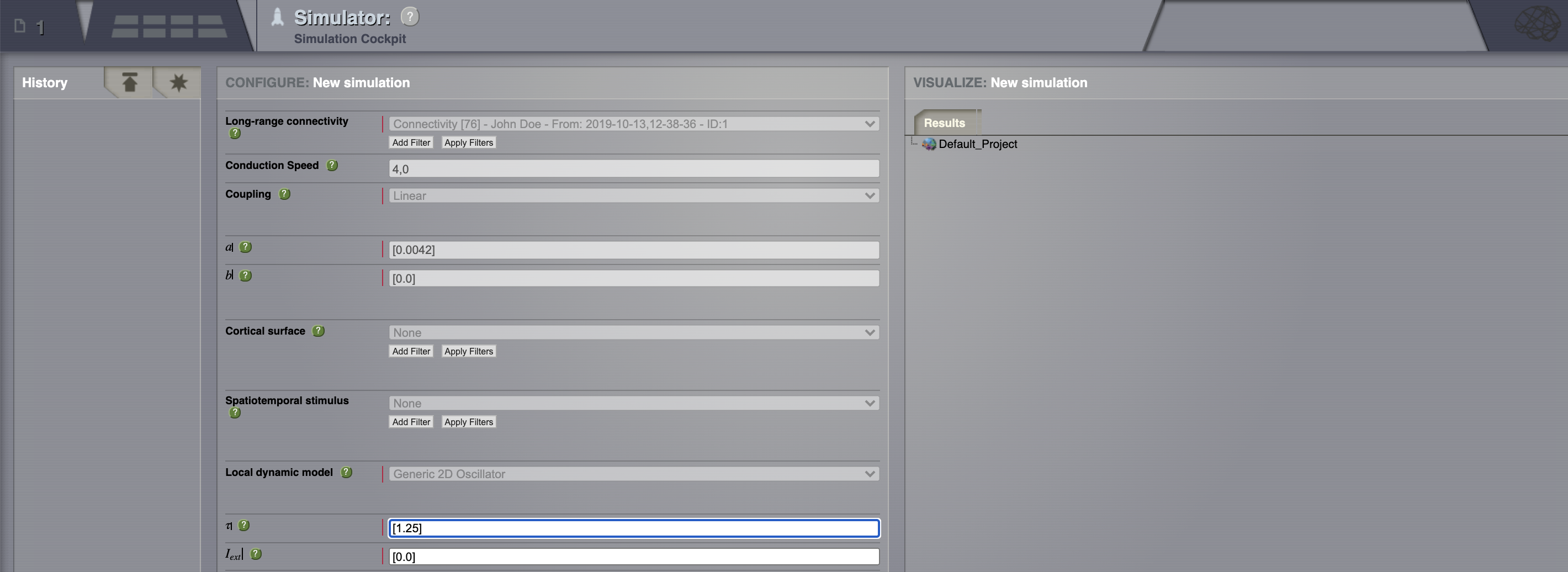
Connectivity: define some structure for your network. Here, we’ll rely on TVB’s default matrix.
Conduction speed: alter the speed of signal propagation through the network to 4 mm/ms.
Set a Long range coupling function. For our present purposes, we happen to know that for the parameters we will use through TVB’s default Connectivity matrix, a linear function with a slope of \(\mathbf{a=0.0042}\) is a reasonable thing to use.
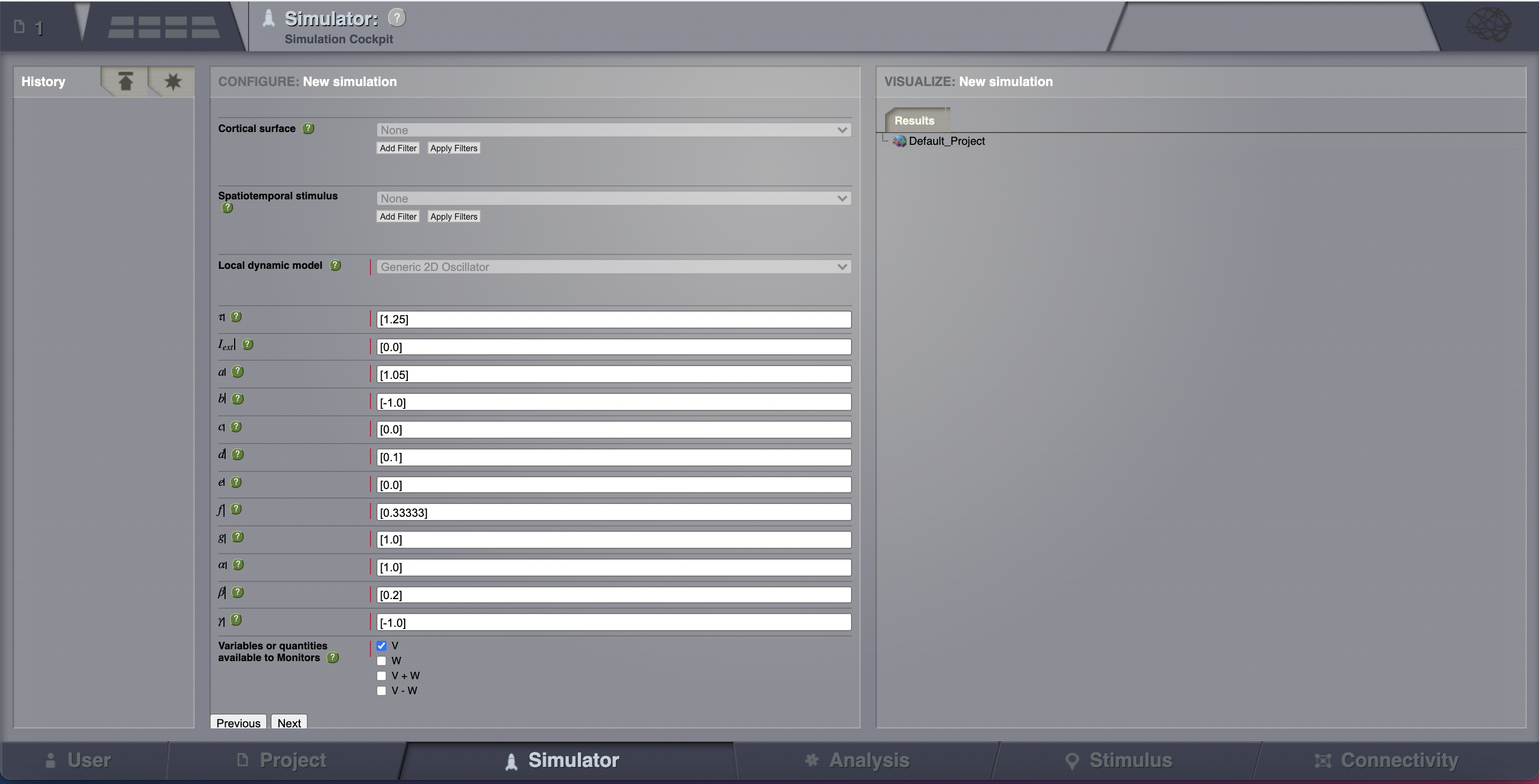
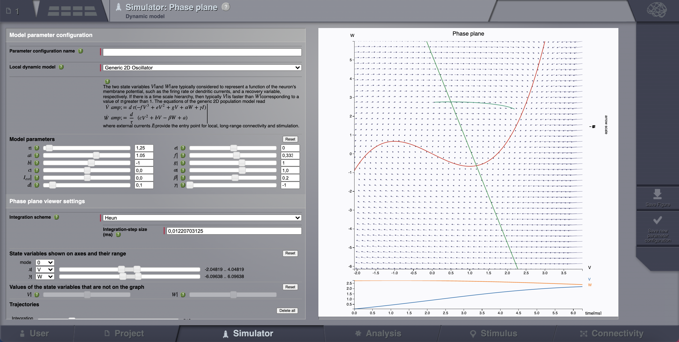
Local dynamics: then define a Model for the local dynamics. Here we’ll use the generic 2 dimensional oscillator with the parameters shown in the following table.
Model parameter |
Value |
\(\tau\) |
1.25 |
\(I_ext\) |
0.0 |
\(a\) |
1.05 |
\(b\) |
-1.0 |
\(c\) |
0.0 |
\(d\) |
0.1 |
\(e\) |
0.0 |
\(f\) |
0.33333 |
\(g\) |
1.0 |
\(\alpha\) |
1.0 |
\(\beta\) |
0.2 |
\(\gamma\) |
-1.0 |
Now that we’ve defined our structure and dynamics we need to select an integration scheme. We’ll use Heun. The most important thing here is to use a step size that is small enough for the integration to be numerically stable. Here, we chose a value of dt = 0.1 ms.
Select the Temporal Average monitor. It averages over a time window of length sampling period returning one time point every period. It also, by default, only returns those state-variables flagged in the Models definition as Model Variables to watch. For our example the Monitor’s sampling period is 1 ms.
Although there are monitors which apply a biophysical measurement process to the simulated neural activity, such as EEG, MEG, SEEG, etc., here we’ll select only one simple monitor just to show the idea. The Raw Monitor takes no arguments and simply returns all the simulated data.
Provide the simulation length. Here we’ll use the default value of 1000 ms.
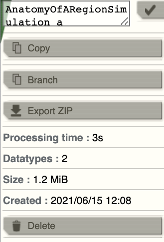
Choose a simulation name. In this example, we chose AnatomyOfARegionSimulation_a.
Click on the Launch button.
Looking at the Results
Go to Projects > Operations dashboard.
Click on the icon of the time-series
 . From the metadata
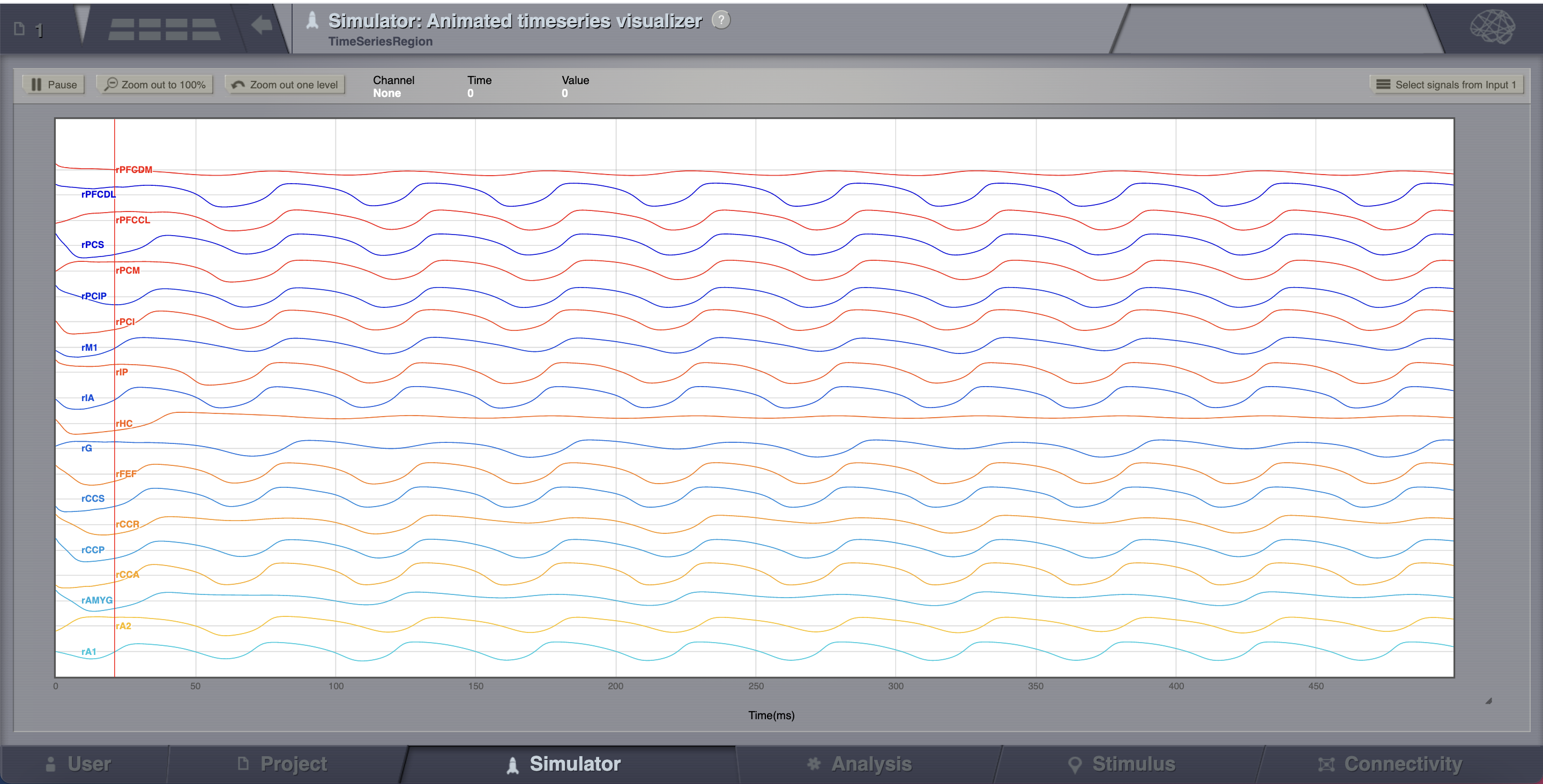
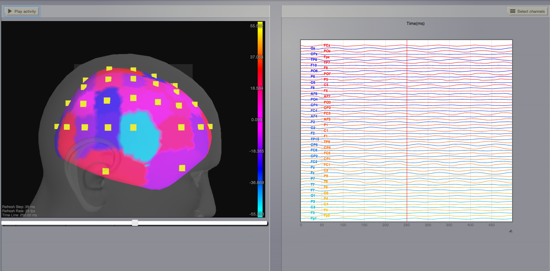
overlay’s visualizers tab, launch the Animated Time Series Visualizer.
. From the metadata
overlay’s visualizers tab, launch the Animated Time Series Visualizer.
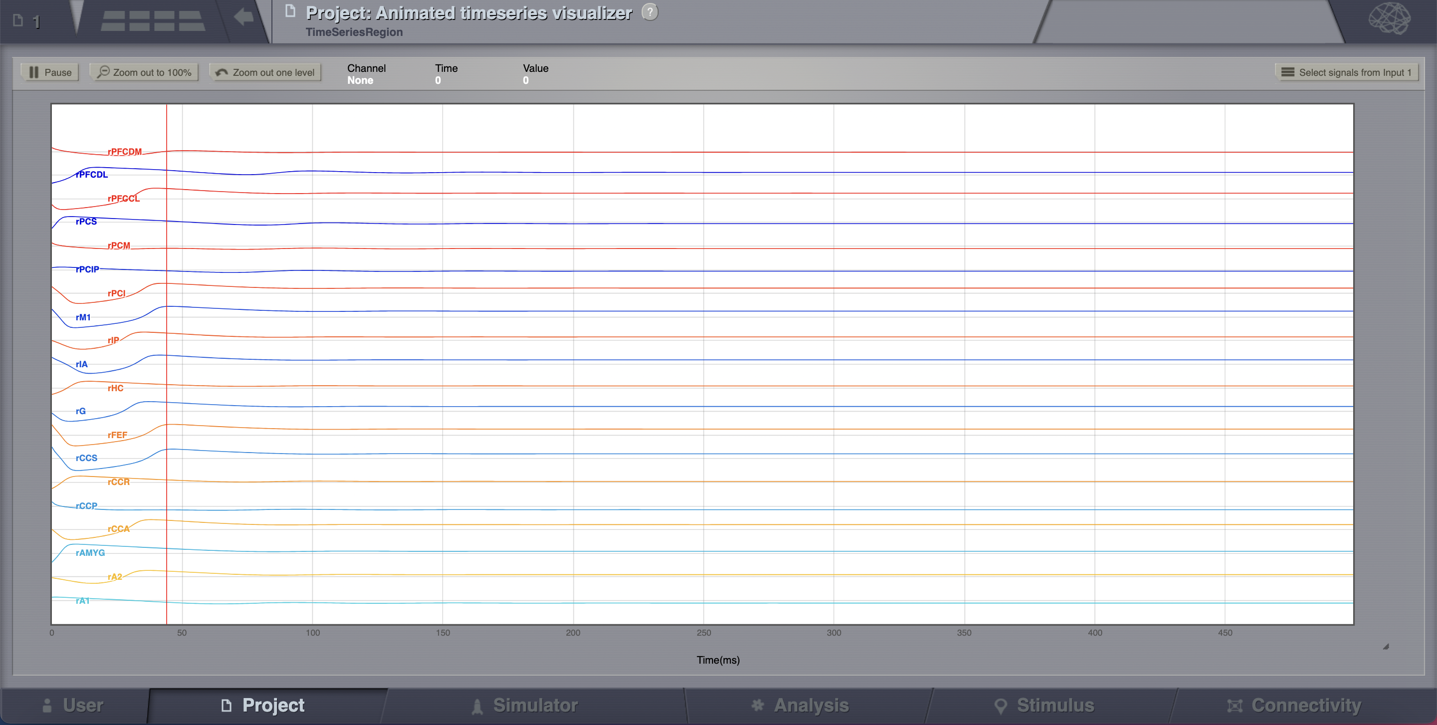
The transient large amplitude oscillatory activity at the beginning of the simulation is a result of the imperfectly set initial conditions.
The initial history (i.e., initial conditions) is merely set by default to be random walks within the general range of state-variables values expected from the model. As the current simulation is configured with fixed point dynamics, if we were to set the initial conditions exactly to the values corresponding to that fixed point there would be no such initial transient (we will see how to achieve that later on).
Now let’s have a look at a second simulation, which has the same parameters as AnatomyOfARegionSimulation_a except that the coupling strength has been increased by an order of magnitude. Hence, the slope of the linear coupling function is \(\mathbf{a=0.042}\).
To make things easy, we copy the first simulation by clicking on
 on the top right
corner of a simulation tab. From the menu you can get a copy, edit the name of the
simulation, branch from it (more about this later), export it as a ZIP file or delete it.
on the top right
corner of a simulation tab. From the menu you can get a copy, edit the name of the
simulation, branch from it (more about this later), export it as a ZIP file or delete it.
Change the name of the new simulation (e.g., AnatomyOfARegionSimulation_b ) and set the coupling strength to the value specificed in step 3. Launch the simulation.
Looking at the time series of AnatomyOfARegionSimulation_b, we can see that the system exhibits self-sustained oscillations.
A frequent question is at which value of coupling strength this “bifurcation” occurs. Well, we can easily set up a parameter search by defining a range of values that will be explored. We’ll see how to do this in the section after the next one.
Analyze the simulation results
Go to the Analysis page. Here you are going to see a list of the basic analyzers.
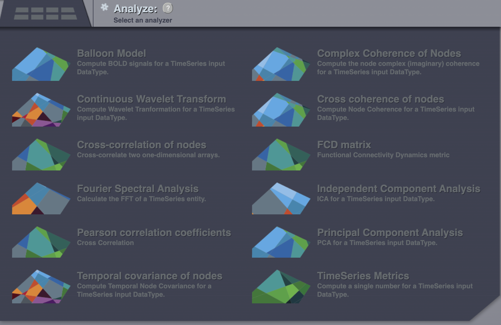
Click on Fourier Spectral Analysis.
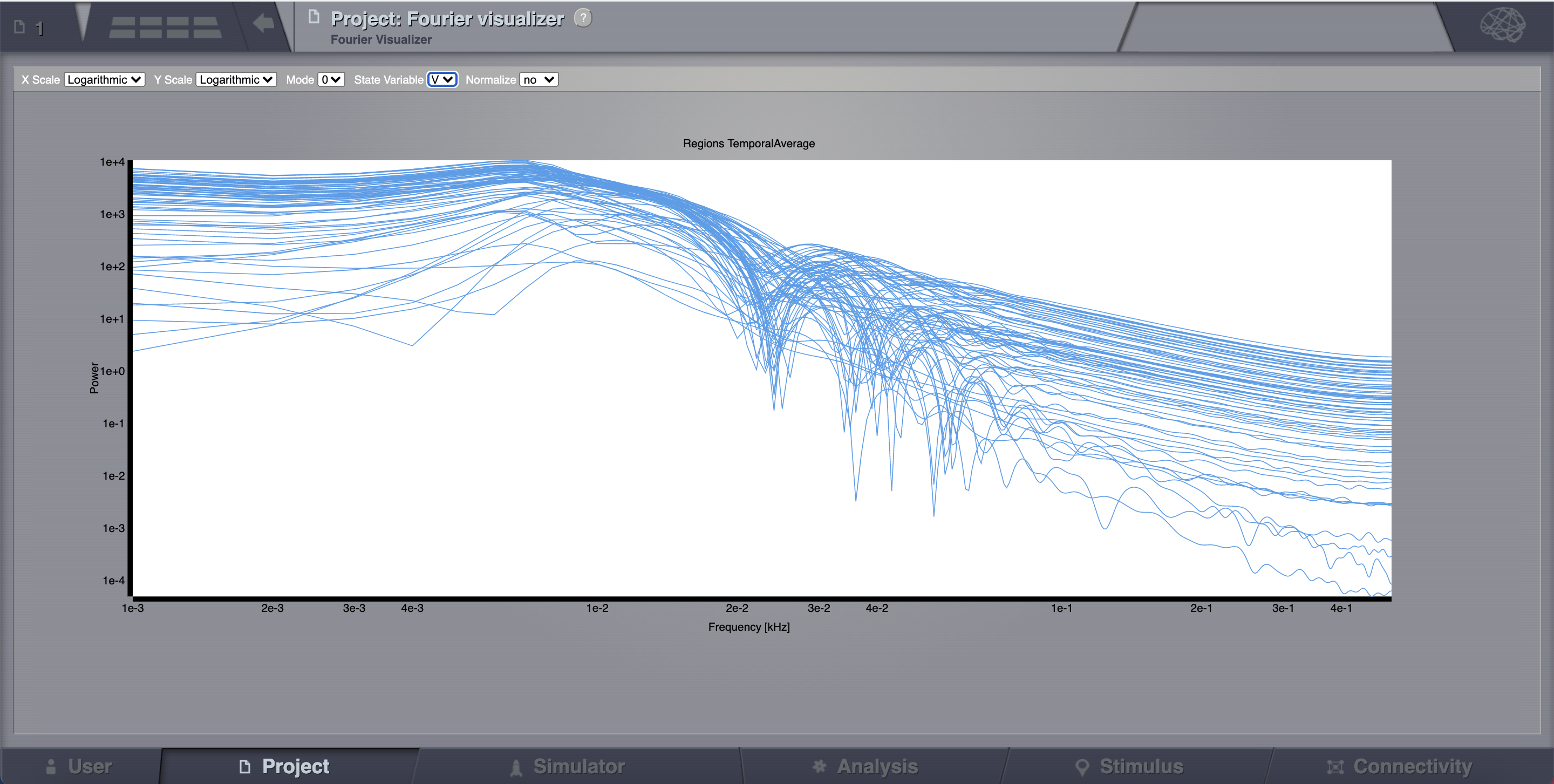
Launch the analyzer with the default parameters.
Look at the results using the Fourier Visualizer.
Parameter Space Exploration (PSE)
A PSE simulation means that TVB will launch a simulation for every value from a range specified of one or two chosen parameters.
Copy the AnatomyOfARegionSimulation_b and name the new simulation AnatomyOfARegionSimulation_pse.
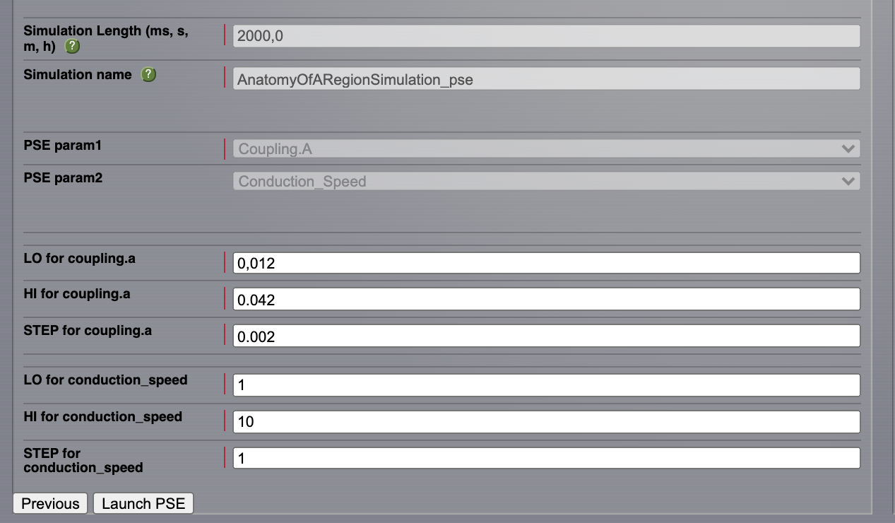
Set the simulation length to 2000 ms.
Click on the Setup PSE button.
Select Coupling.A as PSE param1 and Conduction_Speed as PSE param2. Click on Next.
For Coupling.A set the range between \(\mathbf{0.012 \text{ and } 0.042}\) and the step to \(\mathbf{0.002}\).
For Conduction_Speed set the range between \(\mathbf{1-10}\) and the step to 1 mm/ms.
Click on the Launch PSE button.
All the 135 simulations are presented as a discrete 2D map or a continous pseudocolor map.
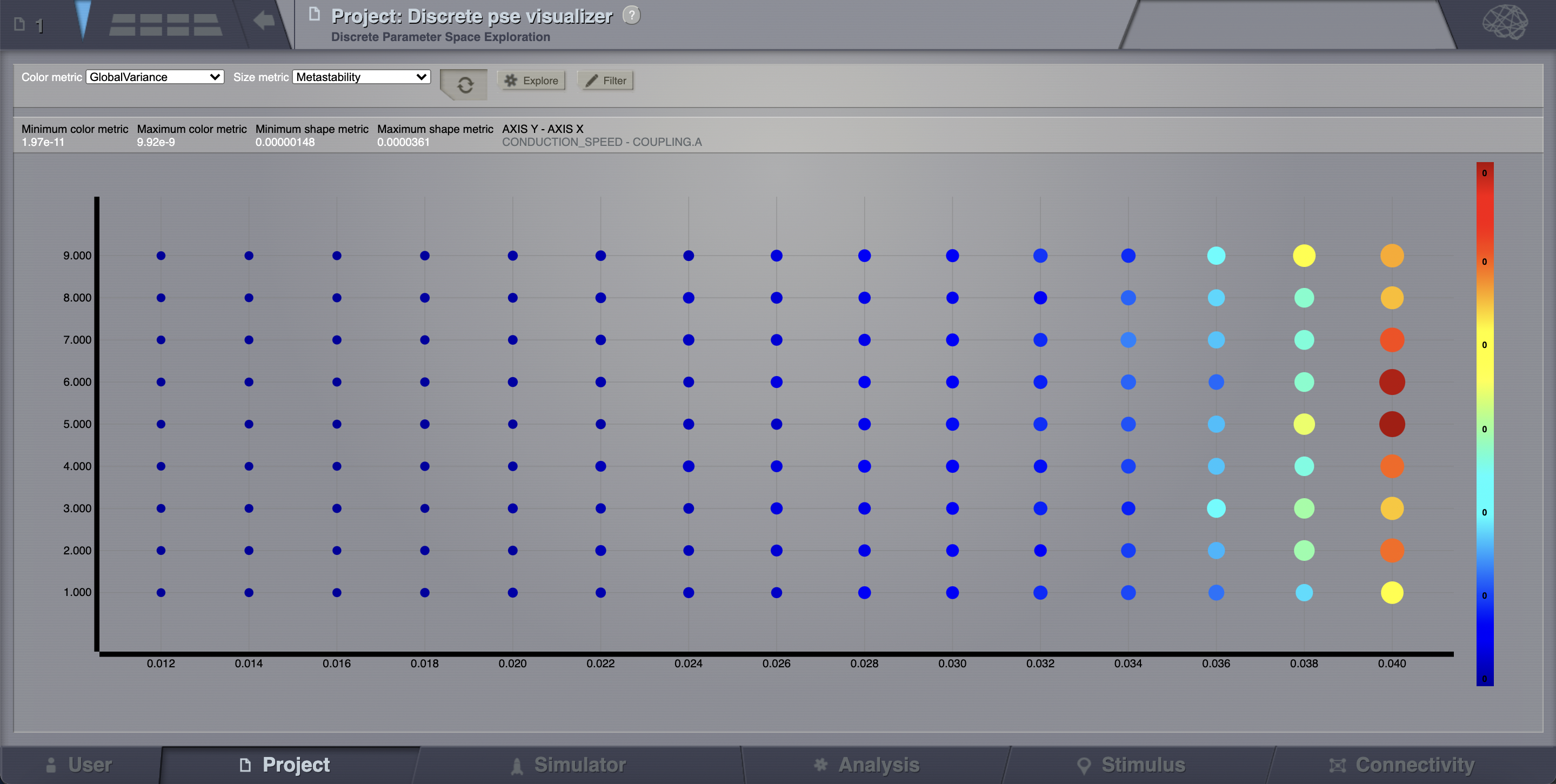
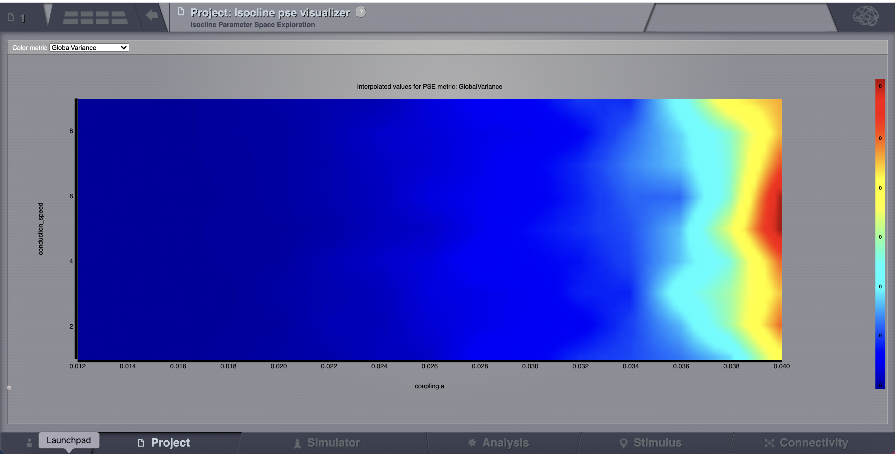
These results are similar to those presented in Ghosh_et_al and Knock_et_al.
Simulation continuation or Branching
Other parameters could be adjusted as well. We mentioned before that the big transient at the beginning of the time-series is due to the initial conditions. To overcome this issue we have a couple of alternatives. First, we could narrow the range of the state variables around the values of a fixed point. How can we know this value?
Clik on
 > Phase plane, you’ll be redirected to a new working area.
In this area there’s an interactive tool, the Phase Plane, which allows you to understand the local dynamics, that is the dynamics of a single isolated node, by observing how the model parameters change its phase plane.
Reset the same parameters as in the table above, click on any point of the phase plane. A trajectory will be drawn. We see that the fixed point is approx (V, W) = (0.0, 2.75)
However, there certainly is a more elegant way.
Set your model with fixed point dynamics and a weak coupling strength (e.g., AnatomyOfARegionSimulation_a)
Run a simulation for 1000 ms.
TVB has a branching mechanism that allows you to use the data of a simulation as the initial history for a new simulation. The only thing you need to know is that the spatio-temporal structure of the network should remain unchanged (e.g., the number of nodes, conduction speed, the recorded state-variables, integration time-step size and selected monitors should be the same).
In AnatomyOfARegionSimulation_a click on
, click on the Branch
button. Click on the Previous button until you get to the second fragment
where you have the coupling params. Set \(\mathbf{a=0.042}\) in the
long-range coupling function.
Stochastic Simulations
As a next step, we will show the basics of running a simulation driven by noise (i.e., using a stochastic integration scheme). Here we’ll also use a region level simulation, but the considerations for surface simulations are the same. In a stochastic integration scheme Noise enters through the integration scheme.
Here we’ll define a simple constant level of noise that enters all nodes and all state variables, however, the noise is configurable on a per node and per state variable level, and as such the noise can be reconfigured to, for example, only enter appropriate state variables of certain thalamic nodes, thus emulating a very crude model of external inputs to the brain.
The Noise functions are fed by a random process generated by a pseudo-random number generator (PRNG). The random processes used have Gaussian amplitude and can potentially be given a temporal correlation. The random process is defined using two parameters plus the seed of the PRNG. The two parameters are: \(\mathbf{D}\), defining the standard deviation of the noise amplitude; and \(\boldsymbol{\tau}\) which defines the correlation time of the noise source, with \(\boldsymbol{\tau = 0}\) corresponding to white noise and any value greater than zero producing coloured noise.
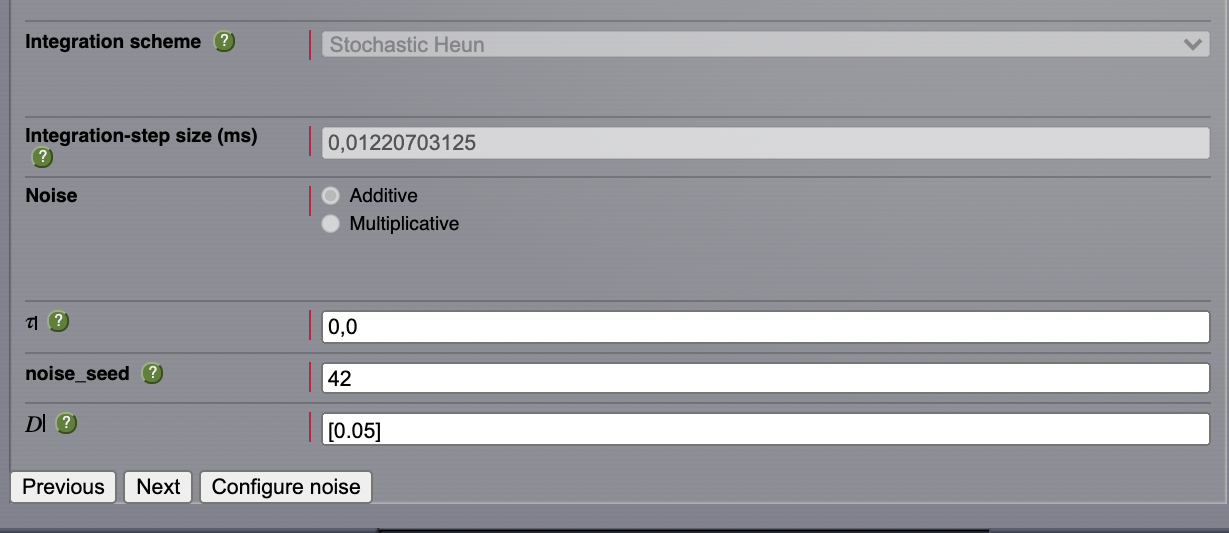
After configuring a model similar to the one presented in AnatomyOfARegionSimulation_b, we select Stochastic Heun as our integration scheme.
Set the values for \(\boldsymbol{\tau=0}\) and noise_seed=42.
Set the noise dispersion, \(\mathbf{D=0.005}\)
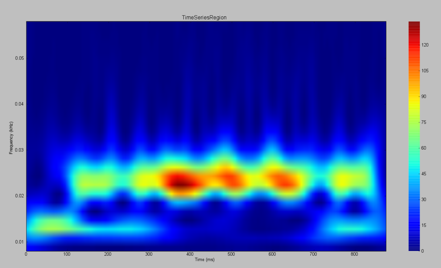
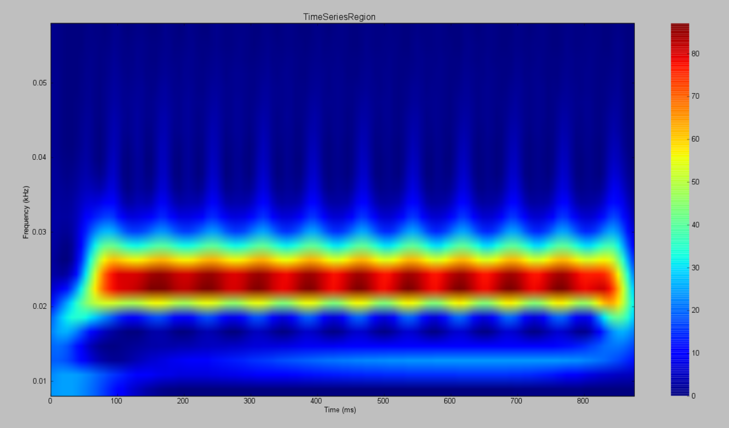
AnatomyOfARegionSimulation_b and AnatomyOfARegionSimulation_stochastic have the same parameters but the latter has an extra background noisy input.
Observe the differences using the Spectrogram of the Wavelet Transform.
Modeling the Neural Activity on the Folded Cortex
This extends the basic region simulation to include the folded cortical surface to the anatomical structure on which the simulation is based. If you haven’t read or followed the information written above, you probably should do that now as here we only really discuss in detail the extra components that are specific to a simulation on the cortical surface.
In addition to the components discussed for a region simulation here we introduce three major components, that is:
Cortical Surface, which is a mesh surface defining a 2d representation of the convoluted cortical surface embedded in 3d space.
Local Connectivity, that represents the probability of the interactions between neighbouring nodes on a local patch.
Region Mapping, a breakup that defines to which anatomical region in the Connectivity each vertex of the mesh belongs to.
The connectivity, speed, coupling strength and and its parameters are the same described in AnatomyOfARegionSimulation_b].
Select the TVB’s default Cortical Surface, which has 16384 nodes.
We rely on TVB’s default Local Connectivity.
Rescale the Local Connectivity with Local coupling strength equal to \(\mathbf{0.1}\).
For the integration we’ll use Heun. Here, integration time step size is the default: \(\mathbf{dt=0.1220703125}\)ms.
The first significant thing to note about surface simulations is that Monitors certainly make a lot more sense in this context than they do at the region level, and so we’ll introduce a couple of new Monitors here.
The first of these new Monitors is called SpatialAverage. To select several monitors just make sure you check the right boxes.
The second of these new monitors, which is an instantiation of a biophysical measurement process, is called EEG. The third will be the already known Temporal Average monitor.
The Sampling period (ms) for all three monitors is 1.953125 ms which is equivalent to a sampling frequency of 256 Hz.
The simulation length is 500 ms.
Lastly, the simulation name is AnatomyOfASurfaceSimulation .
Run the simulation.
- Once the simulation is finished, without changing any parameters,
launch a branch from it with the name AnatomyOfASurfaceSimulation_branch1.
The first of these new Monitors that we mentioned will average over the space (nodes) of the simulation. The basic mechanism is general, in the sense that the nodes can be broken up into any non-overlapping, complete, set of sets. In other words, each node can only be counted in one collection and all nodes must be in one collection.
The second of these new Monitors, EEG, hopefully also unsurprisingly, returns the EEG signals resulting from the simulated neural dynamics using, in the process, a lead-field or Projection Matrix.
EEG signals measured on the scalp depend strongly on the location and orientation of the underlying neural sources, which is why this monitor is more realistic and useful in the case of surface based simulations – where the simulation is run on the explicit geometry of the cortex, which can potentially have been obtained from a specific individual’s brain. In addition, a simulation being built on the specific anatomical structure of an individual subject, the specific electrodes used in experimental work can also be incorporated, providing a link between simulation and experiment.
Define Your Own Local Connectivity
The regularized mesh can support, in principle, arbitrary forms for the local connectivity kernel. Coupled across the realistic surface geometry this allows for a detailed investigation of the local connectivity’s effects on larger scale dynamics modeled by neural fields.
Go to Connectivity > Local Connectivity. In this area we’ll build two different kernels: a Gaussian and a Mexican Hat kernel. We’ll start with the Gaussian kernel.
Select the equation defining the spatial profile of your local connectivity. Here, we’ll set sigma to 15 mm.
Ideally, you want the function to have essentially dropped to zero by the cutoff distance. The cutoff distance, that is, the distance up to which a given node is connected to its neighbourhood (Spiegler_et_al, Sanz_Leon_et_al) is set to 40 mm.
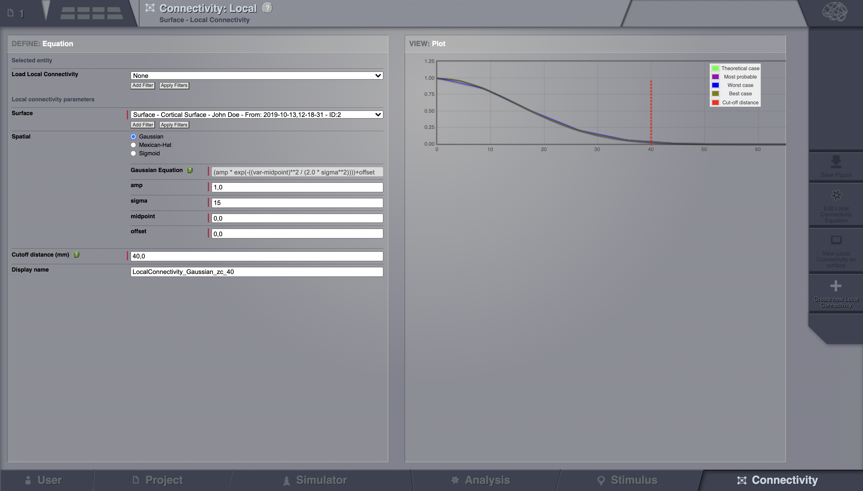
Name your Local Connectivity and save it by clicking on Create new Local Connectivity on the bottom right corner.
This data structure is saved under the name LocalConnectivity_Gaussian_zc_40.
Select the Mexican Hat equation. Here, we changed the default parameters. See the values in the following Table.
Parameter |
Value |
midpoint_1 |
0 mm |
midpoint_2 |
0 mm |
amp_1 |
2 au |
amp_2 |
1 au |
sigma_1 |
5 mm |
sigma_2 |
15 mm |
cutoff distance |
40 mm |
Save your new local connectivity.
This data structure is saved under the name LocalConnectivity_MexicanHat_zc_40.
Finally, we will run two more simulations using different local connectivity kernels.
Copy AnatomyOfASurfaceSimulation.
Change the local connectivity to *LocalConnectivity_Gaussian_zc_40* and set the local connectivity strength to 0.001. Run the simulation.
Copy again AnatomyOfASurfaceSimulation.
This time select *LocalConnectivity_MexicanHat_zc_40*. The local connectivity strength is set to -0.001. Run the simulation.
More Documentation
And that’s it for this session, while the simulations are not
particularly scientifically interesting, hopefully it gave you a sense
of the anatomy of a simulation within TVB and many of the configurable
parameters and output modalities. Online help is available clicking on
the  icons next to each entry. For more documentation on The
Virtual Brain, please see the following articles
icons next to each entry. For more documentation on The
Virtual Brain, please see the following articles
Support
The official TVB website is www.thevirtualbrain.org. All the documentation and tutorials are hosted on http://docs.thevirtualbrain.org. You’ll find our public repository at https://github.com/the-virtual-brain. For questions and bug reports we have a users group https://groups.google.com/forum/#!forum/tvb-users
Ghosh A, Rho Y, McIntosh AR, Kötter R, Jirsa VK. Noise during rest enables the exploration of the brain(s dynamic repertoire. PLoS Computation Biology, 4(10), 2008
Sanz-Leon P, Knock SA, Woodman MM, Domide L, Mersmann J, McIntosh AR, Jirsa VK. The virtual brain: a simulator of primate brain network dynamics. Frontiers in Neuroinformatics, 7:10, 2013.
Spiegler A, Jirsa VK. Systematic approximation of neural fields through networks of neural mases in the virtual brain. Neuroimage, 83C:704-725, 2013
Knock SA, McIntosh AR, Sporns O, Kötter R, Hagmann P, Jirsa VK. The efect of physiologically plausible connectivity structure on local and global dynamics in large scale brain models. Journal of Neuroscience Methods, 183(1):86-94, 2009